Noise Simulation for Gravitational Waves Detector (Virgo, INFN)

The code is adapted from this notebook available on the Virgo use case’s repository.

To know more on the interTwin Virgo Noise detector use case and its DT, please visit the published deliverables, D4.2, D7.2 and D7.4.

You can find the relevant code in the use case’s folder on Github, or by consulting the use case’s README:

Integration author(s): Anna Lappe (CERN), Jarl Sondre Sæther (CERN), Matteo Bunino (CERN)

This repository contains code for simulating noise in the Virgo gravitational wave detector. The code is adapted from this notebook available on the Virgo use case’s repository.

Installation

If running the pipeline directly on a node (or from your terminal), first install the required libraries in the pre-existing itwinai environment using the following command:

pip install -r requirements.txt

Training Pipelines

This repository offers two main approaches for training based on the dataset size:

Small Dataset Pipeline

This pipeline allows you to generate a small synthetic dataset on-the-fly as part of the training process. It’s suited for quick tests and debugging where the entire workflow stays self-contained in memory. The dataset generation step can also be skipped for subsequent runs.

To run the entire pipeline, including dataset generation, use the following command:

itwinai exec-pipeline +pipe_key=training_pipeline_small

If you’ve already generated the dataset in a previous run, you can skip the dataset generation step by executing the following command:

itwinai exec-pipeline +pipe_key=training_pipeline_small +pipe_steps=[1,2,3]

This will load the dataset from memory and proceed with the training steps.

Large Dataset Pipeline

The large dataset pipeline is designed to handle massive datasets that are stored on disk. To generate this data, this project includes another SLURM job script, synthetic-data-gen/data_generation_hdf5.sh, which generates a synthetic dataset for the Virgo gravitational wave detector use case.

The synthetic data is generated using a Python script, file_gen_hdf5.py, which creates multiple HDF5 files containing simulated data. We generate multiple files as this allows us to create them in parallel, saving us some time. To do this, we use SLURM job arrays. After generating the files, they are concatenated into a single, large file using concat_hdf5_dataset_files.py.

To generate a new dataset, you can run the SLURM script with the following command:

sbatch synthetic_data_gen/data_generation_hdf5.sh

Once the dataset is generated, you can proceed with training:

itwinai exec-pipeline +pipe_key=training_pipeline

mlflow ui --backend-store-uri mllogs/mlflow

# In background
mlflow ui --backend-store-uri mllogs/mlflow > /dev/null 2>&1 &

Training using SLURM

If you wish to train the model using SLURM, you can use the itwinai SLURM script builder with the following command to generate a preview of the script:

itwinai generate-slurm -c slurm_config.yaml --no-save-script --no-submit-job

If you are happy with the SLURM script, you can run it either by removing --no-submit-job and let the builder submit it for you, or you can remove --no-save-script—allowing the builder to store the script for you—and then running the script yourself using sbatch <path/to/script>.

Scaling Tests and “runall”

Scaling tests provide information about how well the different distributed strategies scale. We have integrated them into this use case and you can run them using the slurm.py file. The format is very similar to the itwinai generate-slurm command, and you can even pass it the configuration file, but it will overwrite some of the parameters automatically—such as std_out, err_out and job_name.

You can run all strategies by setting --mode to runall and you can run scaling tests by setting --mode to scaling-test and specifying scalability_nodes in the configuration.

To generate the plots, refer to the Scaling-Test Tutorial.

Running HPO for Virgo on JSC

Hyperparameter optimization (HPO) is integrated into the pipeline using Ray Tune and Ray Train. This allows you to run multiple trials and fine-tune model parameters efficiently. HPO is configured to run multiple trials in parallel. There is two methods to run HPO. Both methods are launched with

sbatch slurm_ray.sh

This script sets up a Ray cluster and runs the script for hyperparameter tuning. Change the run command in slurm_ray.sh to run the script you want. You have two options:

1. You can run non-distributed HPO by using the command

python hpo.py --num_samples 4 --max_iterations 2 --ngpus $num_gpus --ncpus $num_cpus --pipeline_name training_pipeline

at the end of the slurm script. Change the argument num_samples to run a different number of trials, and change max_iterations to set a higher or lower stopping criteria. 3. You can run distributed HPO by using the command

$PYTHON_VENV/bin/itwinai exec-pipeline +pipe_key=ray_training_pipeline

at the end of the slurm script.

Please refer to the itwinai documentation for more guides and tutorials on these two HPO methods.

Scalability Metrics

Warning

The scalability plots in here are outdated, the new plots are similar but are grouped by strategies instead of number of nodes.

Here are some examples of the scalability metrics for this use case:

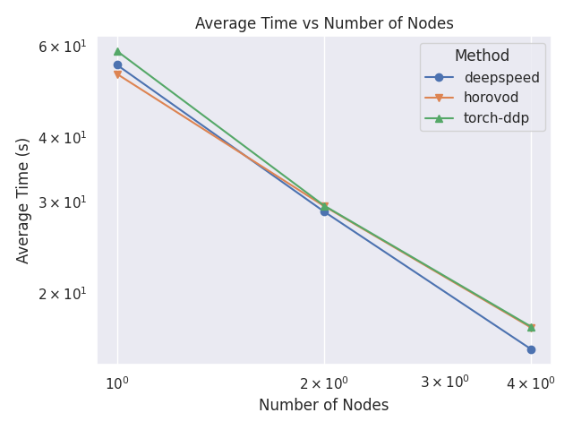
Average Epoch Time Comparison

This plot shows a comparison between the average time per epochs for each strategy and number of nodes.

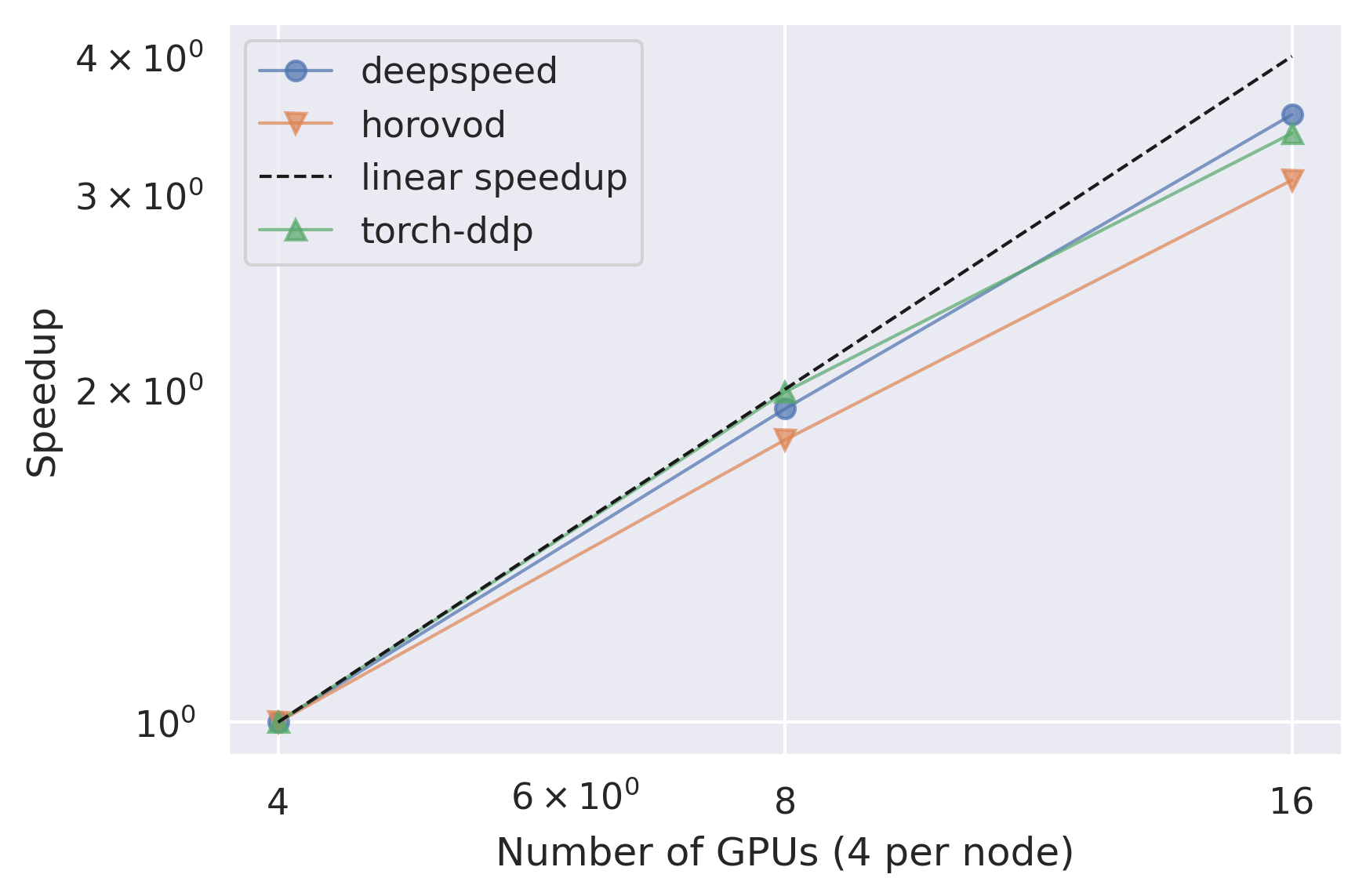
Relative Epoch Time Speedup

This plot shows a comparison between the speedup between the different number of nodes for each strategy. The speedup is calculated using the lowest number of nodes as a baseline.

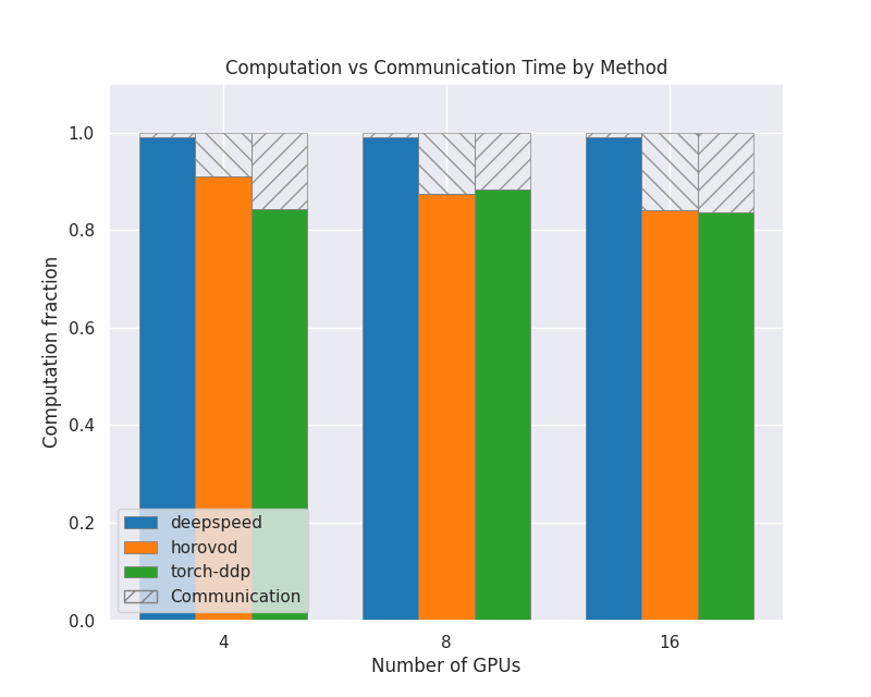
Computation vs Other

This plot shows how much of the GPU time is spent doing computation compared to all the other operations, for each strategy and number of nodes. The shaded area is showing all non-compute operations and the colored area is computation. They have all been normalized so that the values are between 0 and 1.0.

Communication vs Computation

This plot is deprecated and has to be explicitly generated with the –include-communication flag. Computation vs Other is preferred as it is more comparable across different systems. This plot shows how much of the GPU time is spent doing computation compared to communication between GPUs and nodes, for each strategy and number of nodes. The shaded area is communication and the colored area is computation. They have all been normalized so that the values are between 0 and 1.0.

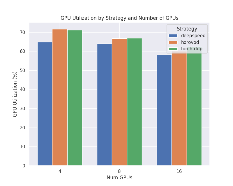
GPU Utilization

This plot shows how high the GPU utilization is for each strategy and number of nodes, as a percentage from 0 to 100. This is the defined as how much of the time is spent in computation mode vs not, and does not directly correlate to FLOPs.

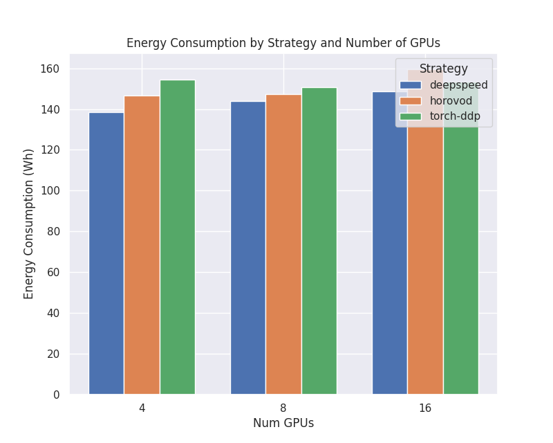
Power Consumption

This plot shows the total energy consumption in watt-hours for the different strategies and number of nodes.